You're building a machine learning model, you've got your features lined up, and then your training results come back looking like garbage. One feature ranges from 0 to 1, another from 0 to 100,000, and your algorithm treats them as if those magnitudes matter. This is where the choice between data normalization vs data standardization becomes critical, and getting it wrong can silently wreck your model's performance.

Both techniques rescale your data, but they do it differently and for different reasons. Normalization compresses values into a fixed range. Standardization centers them around a mean with a unit standard deviation. The right pick depends on your algorithm, your data distribution, and what you're actually trying to accomplish.

This distinction matters especially in healthcare ML, where data pulled from multiple EHR systems arrives in wildly inconsistent formats and scales. At SoFaaS, we handle the integration layer, connecting applications to EHRs like Epic, Cerner, and Allscripts through a unified API, so teams can focus on exactly this kind of downstream data science work instead of fighting infrastructure.

This article breaks down both methods with their formulas, walks through when to use each one, and gives you practical decision criteria for common ML use cases. No hand-waving, just the technical comparison you need to make the right preprocessing call for your next project.

Why feature scaling matters in machine learning

When you feed raw features into a machine learning model, most algorithms treat large numbers as more important than small ones by default. That's not a configuration issue you can toggle off; it's a direct consequence of how gradient-based optimization and distance-based calculations work. A feature measured in thousands dominates a feature measured in single digits, and your model learns the wrong relationships as a result. Understanding where data normalization vs data standardization fits into this problem is how you prevent it from corrupting your model accuracy before training even finishes.

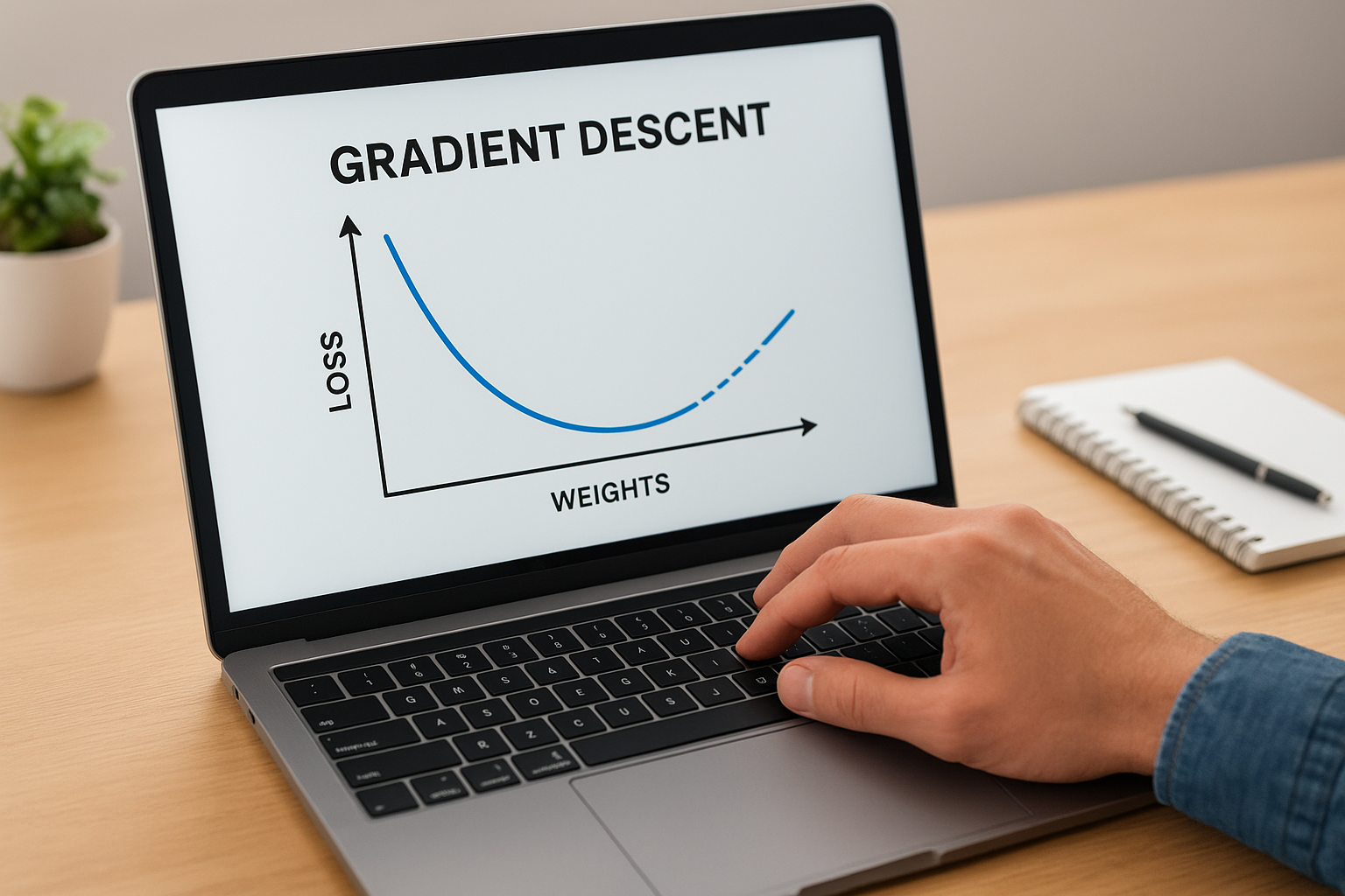
How unscaled features break gradient descent

Gradient descent updates model weights by calculating the gradient of the loss function across all features simultaneously. When your features live on vastly different scales, the loss surface becomes elongated and narrow, creating a valley shape that forces the optimizer to take tiny, inefficient steps toward the minimum. In practice, this means slower convergence, a higher risk of overshooting, and training runs that consume far more compute than necessary. Your learning rate becomes a tug-of-war between features, working fine for one scale while being too aggressive or too conservative for another.

Unequal feature scales can make gradient descent take significantly longer to converge, which compounds directly when you're working with large, multi-source datasets like those pulled from multiple EHR systems.

Beyond convergence speed, neural networks carry built-in weight initialization assumptions that expect inputs within a reasonable numerical range. When you feed in raw data with arbitrary magnitudes, those assumptions break down from the first forward pass, and your network starts training from a badly skewed starting point that is hard to recover from.

How distance-based and decomposition algorithms get distorted

Algorithms like K-nearest neighbors and K-means clustering rely on measuring distances between data points. Euclidean distance squares the difference between feature values before summing them, which means any feature spanning thousands of units completely overwhelms the contribution of features spanning single digits in every single distance calculation. Your clustering model then effectively ignores the smaller-scale feature, not because it's irrelevant, but because its raw numbers are just smaller.

This shows up clearly in healthcare ML, where you might combine patient age (0-100) with lab values running into the thousands. Without scaling, age becomes invisible to the algorithm despite being clinically significant, and your clusters reflect lab magnitudes rather than actual patient similarity.

Principal component analysis (PCA) runs into a related issue. Variance in high-magnitude features dominates the principal components, so PCA finds directions of maximum variance that reflect unit choices from data collection rather than the actual structure of your data. Scaling corrects this by giving every variable equal standing before the decomposition runs.

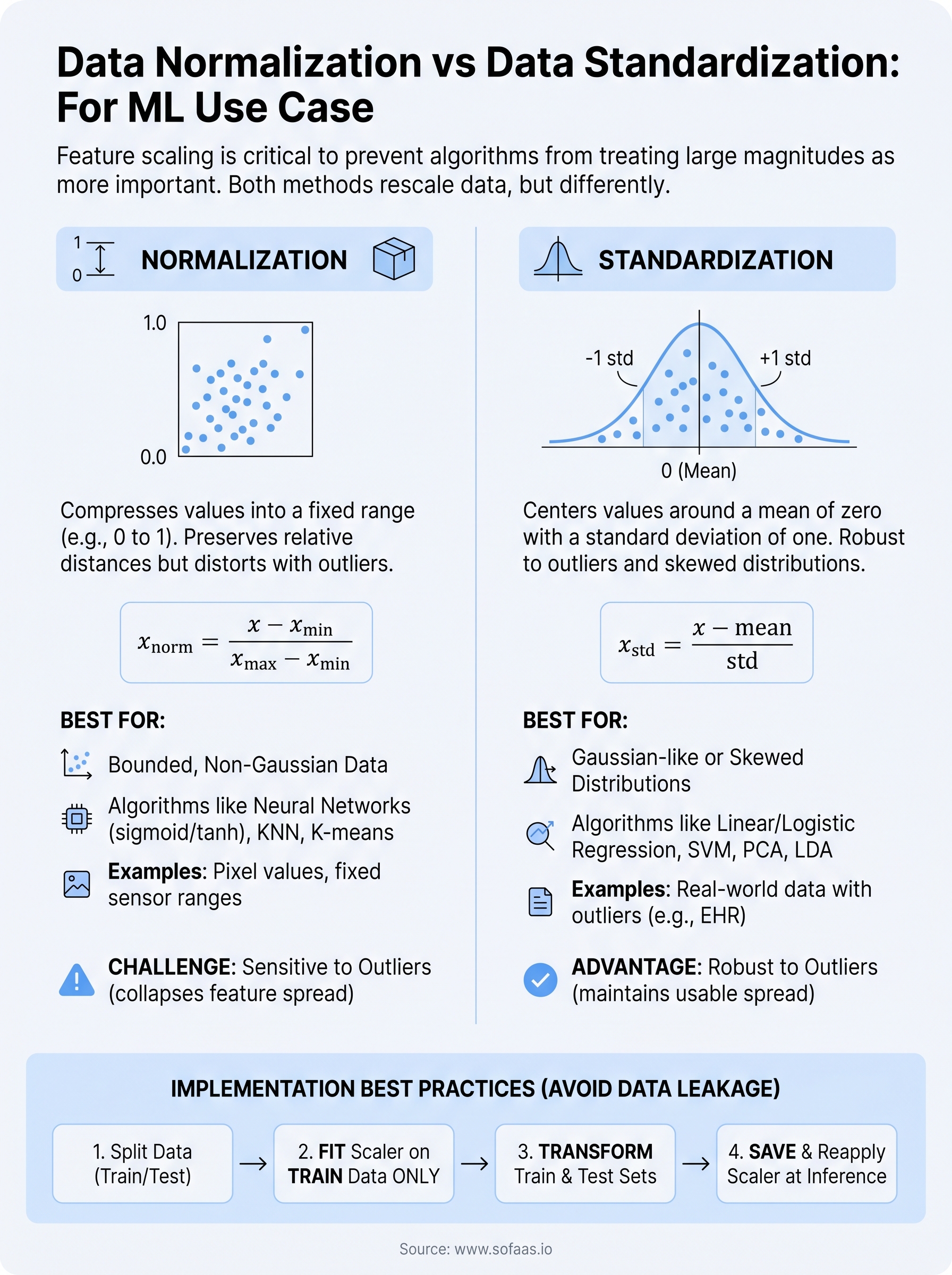
What normalization means and when to use it

Normalization rescales your feature values into a fixed range, most commonly between 0 and 1. The formula subtracts the minimum value of the feature from each data point, then divides by the total range: x_norm = (x - x_min) / (x_max - x_min). Every value maps proportionally within that range, which preserves relative distances between points while eliminating the distortion caused by absolute magnitude differences.

Normalization is the right default when your data has a known, bounded range and you need predictable output scaling, such as pixel values in image data or sensor readings with defined min and max limits.

When normalization fits your use case

Normalization works best when your data distribution is not Gaussian and you have no reason to assume it is. Algorithms that depend on bounded inputs perform significantly better with normalized data. Neural networks using sigmoid or tanh activation functions expect inputs sitting within a small numerical range, and feeding them raw unbounded values slows training and destabilizes weight updates from the first pass.

Reach for normalization when working with image pixel data (which naturally falls between 0 and 255), fixed-range sensor outputs, or any situation where you know the hard boundaries of your features in advance. K-nearest neighbors also responds well to normalized inputs since the distance calculations stay within a consistent scale across all features.

One place normalization breaks down is when your dataset contains outliers. Because the formula depends entirely on the min and max values, a single extreme value compresses everything else into a narrow slice of the target range, destroying the signal you are trying to preserve. That is exactly where the data normalization vs data standardization comparison shifts clearly toward standardization, which is far less sensitive to extreme values and handles skewed distributions without collapsing your feature spread.

What standardization means and when to use it

Standardization transforms your feature values so they have a mean of zero and a standard deviation of one. The formula subtracts the feature mean from each data point, then divides by the standard deviation: x_std = (x - mean) / std. Unlike normalization, this approach does not compress values into a fixed range. Instead, it repositions your data relative to its own distribution, which makes it much more robust when outliers or skewed values are present.

Standardization is the right choice when your data distribution is approximately Gaussian or when your algorithm makes explicit statistical assumptions about the input features.

When standardization fits your use case

Standardization performs best with algorithms that assume normally distributed features or compute statistics based on variance. Linear regression, logistic regression, and support vector machines all fall into this category. These models optimize weights using coefficients that carry statistical meaning, and they produce more stable, interpretable results when every feature sits on a common z-score scale. When you are comparing the data normalization vs data standardization decision for regression tasks, standardization almost always wins.

Your dataset likely contains outliers if you are pulling from real-world sources like EHR systems, where missing data, measurement errors, and extreme clinical values show up regularly. Because standardization uses the mean and standard deviation rather than the min and max, a single extreme value does not collapse your entire feature range the way it does with normalization. The outlier shifts the mean and standard deviation slightly, but the rest of your data retains a usable spread.

Principal component analysis (PCA) and linear discriminant analysis (LDA) both depend on variance-based calculations that assume equal feature contribution. Applying standardization before either of these decomposition methods ensures your components reflect the actual structure in your data rather than an artifact of which units your source system happened to use during data collection.

How to choose between normalization and standardization

The data normalization vs data standardization decision comes down to two things: what your algorithm expects and what your data actually looks like. No single method works universally, so instead of defaulting to one or the other, you need to run a quick diagnostic on both your model choice and your feature distributions before you touch a single value.

Match your scaling method to your algorithm

Your algorithm is the fastest signal for which direction to go. Gradient-boosted trees and random forests are generally scale-invariant because they make decisions based on rank order, not absolute values, so you can often skip scaling entirely for these models. For everything else, the algorithm's internal mechanics tell you exactly what it needs.

Algorithm	Preferred Scaling
Neural networks (sigmoid, tanh)	Normalization
Linear / logistic regression	Standardization
SVM	Standardization
K-nearest neighbors	Normalization
PCA / LDA	Standardization
K-means clustering	Normalization

When you are unsure, standardization is the safer default for most statistical and linear models, while normalization works better for bounded-input architectures.

Match your scaling method to your data distribution

Once you know your algorithm's preference, look at your actual feature distributions. If your features follow a roughly Gaussian distribution with no hard boundaries, standardization preserves that shape and handles the spread correctly. If your features are bounded and uniform, normalization gives you a clean, proportional rescaling without making assumptions about the underlying distribution.

Outliers are the clearest tie-breaker. Real-world healthcare data, financial records, and sensor feeds almost always contain extreme values. In those cases, normalization will compress your entire feature range around that outlier, while standardization absorbs the impact across the mean and standard deviation without destroying the rest of your signal. When your data comes from multiple source systems with inconsistent collection practices, default to standardization unless you have confirmed, bounded ranges.

How to implement scaling safely in an ML pipeline

Knowing whether to use normalization or standardization covers only half the problem. The other half is applying your chosen method correctly without leaking information from your test set into your training process. A mistake here means the data normalization vs data standardization decision you made earlier produces inflated evaluation metrics that fall apart in production.

Fit on training data only, then transform

The most common scaling mistake is fitting your scaler on the entire dataset before splitting into train and test sets. When you calculate statistics across all your data, your test set contributes to those numbers, and your model indirectly sees information it should never have touched. Always split your data first, fit your scaler exclusively on training data, and then apply that fitted scaler to transform both sets separately.

Fitting your scaler on the full dataset before splitting is data leakage, and it makes your model appear more accurate than it actually is in production.

Save and reapply your scaler at inference time

Your scaling parameters need to travel with your model into production. If you recalculate scaling statistics at inference time using only incoming request data, you transform inputs against a distribution that bears no relationship to your training data, and predictions degrade immediately. Save your fitted scaler as a serialized artifact alongside your model weights, then apply that exact transformation to every new input before it reaches the model.

Follow these steps for a clean production pipeline:

• Split data into train and test sets first
• Fit scaler on the training set only
• Transform train and test sets using the same fitted scaler
• Serialize the scaler alongside your model weights
• Load both scaler and model together at serving time

Using scikit-learn's Pipeline object chains your scaler and estimator into a single deployable artifact, which prevents any preprocessing step from being skipped or replaced accidentally between training and serving.

Key takeaways and next steps

The data normalization vs data standardization decision is not arbitrary. Normalization works best for bounded inputs and distance-based algorithms, while standardization handles skewed distributions, outliers, and linear models more reliably. Your algorithm choice and your actual feature distributions together give you a clear path to the right method, without guesswork or trial and error.

Implement either method by fitting your scaler on training data only, then serializing it alongside your model weights and applying that same scaler at inference time. Skipping any of those steps introduces data leakage or prediction drift that only surfaces after deployment, when fixing it costs real time and resources.

If you're building a healthcare application and your data pipeline starts at EHR integration, that upstream layer matters just as much. Connect your app to Epic, Cerner, and Allscripts through a unified SMART on FHIR API, and keep your engineering effort focused on the data science work rather than integration infrastructure.